Process Capability Indices

Description

This module discusses the process capability indices that are commonly used as baseline measurements in the MEASURE phase and in the CONTROL phase.

The concept of process capability pertains only to processes that are in statistical control. There are two types of data being analyzed:

CONTINUOUS DATA:

PPM

DPMO

Z-short term and Z-long term scores VARIABLE DATA:

Cpk

Ppk

Cpm

Before and After Capability Roadmap

This download is available to members

Purpose of Process Capability Studies

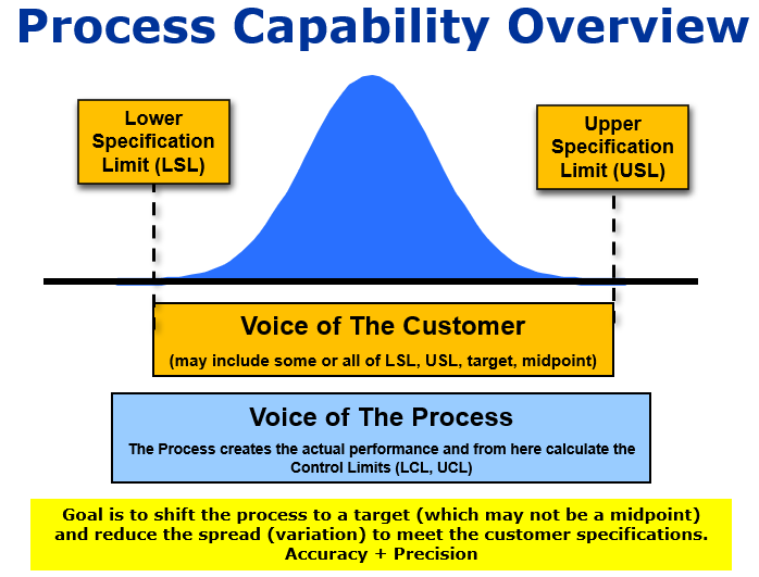
The purpose of studying process capability is to monitor process performance and understand is quantitatively. Furthermore, understand how the performance compares to the VOC (the USL, LSL and possibly a target value).

Capability estimates are strongest (but not always required) when:

Process is stable and in statistical control - use SPC charts to verify

Data is normally distributed*

If not normal, the data is transformable

Satisfies the Central Limit Theorem and normality assumptions apply

Possible Actions

The point of a LSL, USL, and/or target is to compare them to the process capability. The following actions are possibilities once you know you have tracked the process performance

Reduce process variation (the whole premise of Six Sigma)
Center the process or shift if to a Target desired by the customer (may not always be the center of the LSL and USL)
Work with customer to change the LSL, USL, or Target
Do nothing if the process is performing 100% of the time within the specifications or if the nonconforming loss is minimal and acceptable to the customer. The price for perfection can be extreme so sometimes there are acceptable losses.

Considerations

The following are issues to consider when establishing metric-based capability.

Stability

An unstable process makes mean and variability predictions difficult.

Sample Sizes

Inadequate sample sizes may not reflect the actual process.

Normality

Non-normal data may lead to misleading metrics which could lead to wrong decisions. Keep in mind the data does not have to be normally distributed to use control charts. The data does have to fit (or be assumed) a normal distribution to use these capability indices.

DISCUSSION

The capability indices of Ppk and Cpk use the mean and standard deviation to estimate probability. A target value from historical performance or the customer can be used to estimate the Cpm.

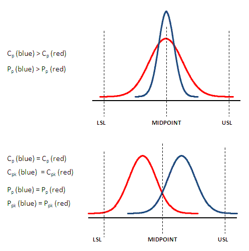
Cp and Pp are measurements that do not account for the mean being centered around the tolerance midpoint. The higher these values indicate the narrower the spread (more precise) of the process. That spread being centered around the midpoint is part of the Cpk and Ppk calculations.

The midpoint = (USL-LSL) / 2

The addition of "k" quantifies the amount of which a distribution is centered. A perfectly centered process where the mean is the same as the midpoint will have a "k" value of 0.

The minimum value of "k" is 0 and the maximum is 1.0.

An estimate for Cpk = Cp(1-k).

and since the maximum value for k is 1.0, then the value for Cpk is always equal to or less than Cp.

Cp and Cpk are coined as "within subgroup", "short term", or "potential capability" measurements of process capability because they use a smoothing estimate for sigma. These indices should measure only inherent variation, that is common cause variation within the subgroup.

Plotting subgroup to subgroup data as individuals (I-MR) will likely show an out-of-control chart and process that is likely in control just showing lot-lot variation, shift-shift variation or day to day variation which is expected.

Therefore, the SEQUENCE of gathering and measuring is mandatory to have a correct calculation of Cp and Cpk. The subgroups should be the same size. The highest value for Cp is most likely achieved when the samples are collected with one operator on one shift on one machine with one set of tools, etc.

Most common estimate for Cp and Cpk uses an average of the subgroup ranges, R-bar, in a process with only inherent variation (no special causes) formula that lowers the width of the data distribution (sigma) from the X-bar & R chart. This optimization of sigma reduces its spread and value further increasing the value Cp and Cpk over Pp and Ppk.

Pp and Ppk use an estimate for sigma that takes into account all or total process variation including special causes (should they exist) and this estimate of sigma is the sample standard deviation, s, applies to most all situations. This estimation accounts for "within subgroup" and "between subgroup" variation.

Cp is a short-term index and not dependent on centering and uses an optimal smoothed and reduced estimate for sigma, represents the process entitlement. Process entitlement the best a process can be expected to perform in terms of minimal variation under existing conditions.

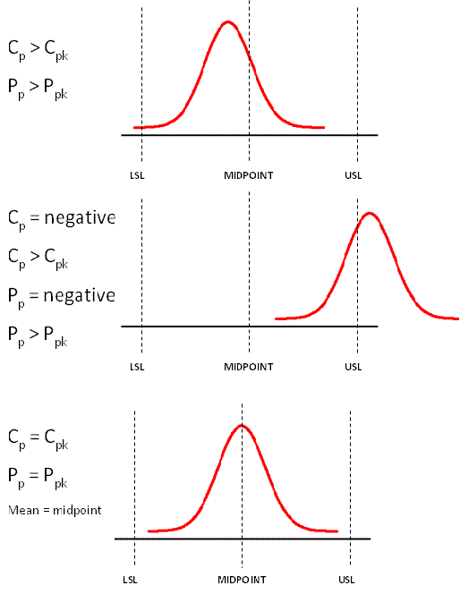
The Cpk value can never exceed Cp. A perfectly centered distribution on the midpoint will have a Cpk = Cp. Any movement either way from the midpoint will have a "k" value of <1.0 and Cpk < Cp.

In Cp and Pp, consider the numerator (USL-LSL) as a constant. As the estimate for standard deviation (sigma) of a distribution reduces and approaches zero the value of Cp and Pp will increase towards infinity.

Cp and Pp are meaningless if only unilateral tolerances are provided, in other words, if only the USL or LSL are provided. Both tolerances (bilateral) must be provided to calculate a meaningful Cp and Pp. A boundary can be used (such as 0 lower limit) but the meaning of Cp to Cpk will differ from the meaning using bilateral tolerances.

The overall process performance indices, Pp and Ppk, most often uses the sample standard deviation, s, formula as an estimate for sigma. There are other methods available for estimating the overall (total) process sigma.

The Cpk and Ppk will require two calculations and selecting the minimum value of those two calculations is the value use as baseline. Use this baseline to compare to customer acceptability level. These can be calculated using unilateral or bilateral tolerances.

The formula for Cpk and Ppk is used with potentially bilateral tolerances (where a LSL and USL are provided). If only one specification is provided (unilateral) then the value used for Cpk and Ppk is provided by the calculation that involves the specification limit provided.

Pp and Ppk are rarely used compared to Cp and Cpk. They should only be used as relative comparisons to their counterparts. Capability indices, Cp and Cpk, should be compared to one another to assess the differences over a period of time. The goal is to have a high Cp, and get the process centered so the Cpk increases and approaches Cp. The same applies for Pp and Ppk.

Cpk and Ppk account for centering of the process among the midpoint of the specifications. However, this performance index may not be optimal if the customer wants another point as the target other than the midpoint. The calculation of Cpm accounts for the addition of a target value.

Capability Analysis for VARIABLE data

STEP 1:

Decide on the characteristic being assessed or measured. Such as length, time, radius, ohms, hertz, watts, volts, thickness, hardness, tensile strength, weight, or distance.

STEP 2:

Validate the specification limits (LSL and USL) and possibly a target value provided by customer.

STEP 3:

Collect and record the data in order at even intervals in the Data Collection Plan. If you are taking multiple readings in a group, then you have subgroups and will need to get the same number of readings at each group. If you have a destructive test such as tensile testing, then you will get one reading per part and the subgroup size is one.

To analyze short and long-term performance there should be 20-25 rational subgroups. Keep in mind what is practical and economical.

You will have to indicate the subgroup size when analyzing the data using statistical software.

STEP 4:

Assess process stability using a control chart such as I-MR, X-bar & R, or other proper control chart. There may be a specific customer required charting method.

STEP 5:

If the process is stable, assess the "normality" of the data. Assuming 95% level of confidence, the p-value should be greater than 0.05. Data must be normal, able to be assumed normal, or transformed to normal data in order to proceed.

STEP 6:

Calculate the basic statistics such as the mean, standard deviation, and variance. Calculate the capability indices (Cp, Cpk, Pp, Ppk, Cpm) as applicable.

STEP 7:

Verify to the customer requirement for capability where the process is acceptable.

NOTE: This is a SAMPLE analysis. These results are used to make inferences about the POPULATION.

Capability Analysis for Attribute Data:

STEP 1:

Gather and record samples

STEP 2:

Count the defects

STEP 3:

Use P chart or U chart to assess process stability

STEP 4:

Calculate the Defect rate such as Proportion Defective if you have Binomial data or DPU if you have Poisson data.

STEP 5:

Analyze the Cumulative probability chart and ensure stability. Gather more samples if necessary.

STEP 6:

Calculate the z-score.

Explaining the Indices

Defining Standard Deviation

In many automotive standards the data is plotted using 125 samples in rational subgroup sizes of 5 on an X-bar & R chart (25 data points on the chart). The R-bar value used in estimation for sigma for Cp and Cpk is the average of each subgroup's range.

The estimation for sigma, s, in Pp and Ppk, is commonly the same formula as the sample standard deviation calculation. It is free from dependency on the sequence of sample gathering and is not a function of the subgroup spreads.

If the parts being analyzed are being pulled out of carton or pallet randomly and the order of production or subgrouping is unknown, then the ONLY estimate is to use the (or one of) "long term" estimate or the "short term" estimate.

It takes into account the total spread of all data points for true performance. However, if the order isn't maintained and measurement plotted vs. time, control charts can't be employed to assess stability and control of the process. Always try to avoid to assessing capability of measurements where process control isn't first understood.

There are many other types of sigma estimates and often statistical software programs allow these choices. There is also much confusion among terminology and the true meaning of the capability indices. The underlying assumptions of control are debatable.

As mentioned before, a control chart of may appear out of control as some of the special cause points may be actual common cause due to inherent operator-operator or shift-shift variability.

Therefore (whenever possible) when assessing process capability, Cp and Cpk, of a manufacturing process (the best it can perform) use only one shift with one operator with same lot of material with same tools on the same machine, etc.

Maintaining the correct sequence gathering and plotting is required for Cp and Cpk. Since Pp and Ppk measure total observation capability the sequence is not as important.

More importantly, select the calculation for estimating the standard deviation and the capability indices that the team and the customer agree on. Use the same calculations and indices throughout the project.

NOTES:

Processes that are in control should have a process capability that is near the process performance. The more significant the gaps between capability and performance the higher the likelihood of special cause data.

It is possible to have data that falls outside the specification limits (LSL, USL) and still have a capable process. It depends on the performance of the other data, and the customer acceptability levels and any specific rules that may apply from the customer, standard, law, or company.

This is all a part of gathering the Voice of the Customer (VOC) and validating the specifications when using them. Due to the dynamics of customer needs and expectations it is important to continually validate the limits and acceptability levels throughout the project. There could be a long period of time between the SIPOC and the development of the Control Plan and assessing final capability and any changes are better captured sooner than later.

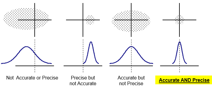
See the graphs shown below to help visually explain the relationships.