Families of Variation (FOV)

From the Data Collection page, we discussed the importance of gathering data across all the FOV's. This is done in the early MEASURE phase before the Measurement System Analysis (MSA).

Let's briefly review the Data Collection process:

When setting up the collection system it is important to collect data only once and minimize the burden on the operators, team, and the GB/BB. Ensure to capture all the families of variation (FOV) that should be analyzed or relevant.

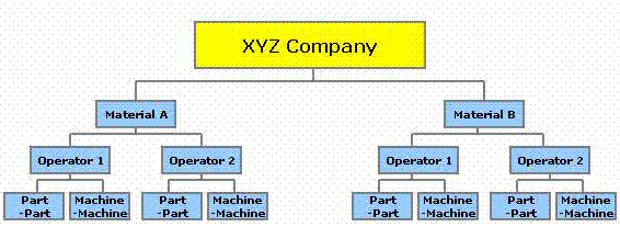
Create a Families of Variation (FOV) diagram.

Think about all the factors that contribute to the process performance (mean and variance). 

The entire amount of variation found in a set of data can be broken down to the variation from the Process + the variation from the Measurement System, which should be calculated from the MSA.

If: The % Study Variation in the MSA was found to be X, the Process Variation = 1 - X.

A FOV diagram evaluates the sources of Process Variation. These sources include families such as:

• Part-Part
• Shift-Shift
• Operator-Operator
• Machine-Machine
• Form-Form
• Material - Material
• Tool-Tool, etc.
  
• Date/Time (almost always important is to collect the time and date)

Example FOV Tree

You should collect at least (too much information is not a bad thing if its easily and readily available) data from every family of variation. 

Another possibility is shown below. Each one of the families will contribute to the overall process performance.

The combination (not necessarily the sum) of all their variances represents the overall process variance. These are all "short" term sources that make up the "long" term variation.

For this discussion on FOV, we will assume all the data has been collected. Furthermore, we will assume the MSA has passed. Therefore, the Six Sigma team can direct all its energy toward the Process performance. 

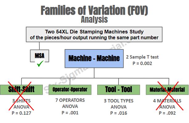
Shown below are the results from an example Six Sigma project that has a goal of improving the output (pieces/hour) of two identical die stamping machines.

They are only looking at the Performance component of OEE. 

FOV with Six-Sigma-Material.com

The Six Sigma BB first compared the mean output of each machine using a 2 Sample T test. Assumed a CL of 95% (alpha-risk of 5% or a critical p-value of 0.05).

The data passed the normality test so the parametric hypothesis test can be applied. 

Now that the data is verified legitimate it is quick and easy to run a battery of hypothesis tests using statistical software.

Lets start by reviewing the Machines to each other

A p-value of 0.002 indicates (reject the H_O) that there is a difference in their means. (This doesn't say anything about the pieces/hour standard deviations for each machine...use the F-test for that review - which is just as important and studying their means). 

POINTER:

As as BB/GB you should be able to run these hypothesis tests, as many as necessary, to give you as much insight as possible. You've already done the hard part and that was gathering the data and passing the MSA.

All you need to now is to select the correct hypothesis test, set up each correctly, enter the data correctly into the software, and interpret the results correctly. This is actually the easy part. 

Now, let's dig deeper into the FOV's of each machine. 

The team gathered data on 3 shifts, from 7 operators, 3 tooling types, and 4 types of raw material. The operators had worked on each shift.

SHIFT-SHIFT study

The Six Sigma BB ran a variety of hypothesis test starting with ANOVA to compare the pieces/hour across the three shifts.

The p-value of 0.127 is >0.05 so it was excluded from further discussion. The shift does not have an impact on the means (maybe it does play a role in the variation).

OPERATOR-OPERATOR study

The p-value of 0.001 is <0.05 so it is a family (or factor) to dig deeper within. There is a statistical difference among operators. 

TOOL-TOOL study

The p-value of 0.016 is <0.05 so it is a family (or factor) to dig deeper within. There is a statistical difference among the three types of tools used to run the part. 

MATERIAL-MATERIAL study

The p-value of 0.092 is >0.05 so it is not a family (or factor). There is not a statistical difference among the three types of materials that were used to make the part. 

What's next?

Keep in mind, everything just discussed was about studying the means. A BB should also study the variation in as many ways as possible. Study the variation in the pieces/hour on each shift, material, tool, and operator as well.

Recall the goal of Lean Six Sigma is to shift the target to a desirable level BUT also reduce the variation in process performance and improve its consistency (predictability). Squeeze the bell curve (with the LSL and USL) and shift the mean to where it needs to be.

The team should discuss inputs that create Operator and Tool performance differences. Consider a Fishbone and Prioritization Matrix to identify which ones are most important on impacting the pieces per hour related to Operator and Tooling.

If feasible, set up a Design of Experiments and find out what combinations are optimal.

But first try to get all the operators on the same level through training, poka-yokes, etc. Then any operators can run with the optimal tooling and material and get the best and consistent results. 

ShareFacebookXWhatsApp

Return to the ANALYZE Phase

Go to Design of Experiments

Six Sigma Job Openings

Six Sigma Templates, Statistics Tables, and Calculators

Six-Sigma-Material Home Page