The Exponential Distribution is continuous distribution commonly used to model waiting times before a given event occurs, or times between random occurrences.

It's also used for products with constant failure or arrival rates. It represents the time between trials in a Poisson process.

If this waiting time is unknown, it can be considered a random variable, x, with an exponential distribution.

Generally, if the probability of an event occurs during a certain time interval is proportional to the length of that time interval, then the time elapsed follows an exponential distribution.

This distribution uses a constant failure rate (lambda) and is the only distribution with a constant failure rate. It is a valuable tool to predict the mean time between failures and plays a significant role in Predictive Maintenance, Reliability Engineering, and Overall Equipment Effectiveness (OEE).

When the downtime can be predicted, not only can it control costs but managing labor becomes easier and machine OEE improves. All three components of OEE (Availability, Performance, Quality) could benefit from effective probability information.

Understanding the probability until a failure or a particular event can be very valuable information. While we all try to read the crystal ball the best we can, any reliable tool to predict the future is powerful for obvious reasons.

Characteristics:

A continuous distribution (Poisson is discrete)
Right-skewed
values of x range from 0 to infinity with the peak always at 0.
curve decreases as x become greater.

Applications include:

mean arrival time of planes at an airport
failure rate of electronic devices
using the mean time of light bulb, calculate probability of life at specified hours.
predicting how long a machine will run before unplanned downtime
how long until the next email comes through your Inbox at work
time until next rainfall
time between phone calls at a call center
length of time of phone calls
how long a battery last

Probability Density Function (PDF)

This is a continuous probability distribution function with formula shown below:

t = time

Lambda (λ) = the failure or arrival rate which = 1 / MBT, also called rate parameter

MBT = the mean time between occurrences which = 1 / λ

and must be > 0

Median time between occurrences = ln(2) / λ

or about 0.693 / λ

Mode = 0

Skewness = 2

Variance (σ²) = of time between occurrences = 1 / λ²= MBT² = mean²

Therefore the standard deviation (σ) = MBT = 1 / λ

Example:

What is the standard deviation of a process with a mean (MBT) of 15.0 and exhibits the exponential distribution?

1) 30.0

2) 15.0

3) 0.067

Answer: 15.0

Cumulative Density Function (CDF)

Example using the CDF

The time between failures in a hemming machine modeled with the exponential distribution has a MBT rate of 112.4 hours. The Six Sigma team has a goal to increase the MBT to greater than or equal to 150 hours.

To help understand the current state, what is the probability that the time until the next failure is less than 150 hours?

Lambda (λ) = 1 / 112.4 = 0.008897

F (time between events is < x) = 1 − e^−λt

F (time between events is < 150) = 1-e^{-0.008897×150} = 1 - 0.263277 = 0.736723

The probability of the hemming machine failing in < 150 hours is 73.7% in its current state. This is a baseline measurement for the team.

NOW WHAT?

In the IMPROVE phase, the team goes on to make several modifications to the machine and collects new data. They show a presentation to others in the company that claims the probability of the time until the next failure has been reduced to <5%.

What must the new minimum MBT rate be at a minimum to achieve this probability of =<5%?

Solve:

We need to work backwards with the data provided and solve for MBT. Start with:

F (time between events is < x) = 1 − e^−λt

Substitute λ with 1 / MBT:

F (time between events is < x) = 1 − e^{−(1 / MBT) * t)}

Substitute F = 0.05 (5%)

0.05 = 1 - e^{-t / MBT}

0.95 = e^{-t / MBT}

ln 0.95 = -t / MBT

-0.05129 = - t / MBT

Substitute t = 150 hours

-0.05129 = - 150 / MBT

MBT = - 150 / -0.05129

MBT = 2,294 hours (or 121.85 full days)

This would mean that the team claims a new MBT rate of AT LEAST 2,294 hours!

We're not sure how many data points they could have collected so this would be some extreme claim from the team.

The key is to not only improve the MEAN but more importantly REDUCE THE VARIATION.

How consistent is the MBT rate at 2,294 hours?

If the failure rate is not consistent (meaning that the failure rate has a high variance and standard deviation) then that represents unreliability and a confidence interval will indicate a better depiction of what will likely occur in the future (using an alpha-risk of 0.05).

The team should present data in terms of central tendency (MBT in this case) but also measures of dispersion and use a confidence interval on the actual "after" data collected.

Comparing Exponential & Poisson Distributions

The Exponential Distribution has a Poisson Distribution when:

1) the event can occur more than 1 time

2) the time between two successive occurrences is exponentially distributed

3) the events are independent of previous occurrences

Both the Poisson Distribution and Exponential Distribution are used to model rates but the latter is used when the data type is continuous.

If the random variable, x, has an Exponential distribution then the reciprocal (1/x) has a Poisson Distribution.

The Poisson Distribution is applied to model the number of events (counts) or occurrence per interval or given period (could be arrivals, defects, failures, eruptions, calls, etc.). This models discrete random variable.

The Exponential Distribution is applied to model the mean time (such as waiting times) between occurrences, time is a continuous variable.

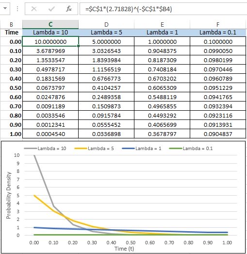
Probability Density Function at various Lambda

Shown below are graphical distributions at various values for Lambda and time (t). The formula in Excel is shown at the top of the figure. They each take on a similar shape; however, as Lambda decreases the distribution does flatten.